Department of Mechanical Engineering, Indian Institute of Technology Madras, 206 Fluid Systems Laboratory, India.
*Corresponding author: Vishal VR Nandigana,
Department of Mechanical Engineering, Indian Institute of
Technology Madras, 206 Fluid Systems Laboratory, Chennai 600036, Tamil Nadu, India.
Email: nandiga@zmail.iitm.ac.in
Received: Aug 01, 2025
Accepted: Sep 29, 2025
Published Online: Oct 06, 2025
Journal: Journal of Artificial Intelligence & Robotics
Copyright: © Nandigana VVR (2025). This Article is distributed under the terms of Creative Commons Attribution 4.0 International License.
Citation: Nandigana VVR. Physics informed neural network to understand multimer. J Artif Intell Robot. 2025; 2(2): 1026.
In this paper we develop physics informed neural network model to obtain parameters of the multimeter design. We design the voltage and current of the multimeter. We consider fixed geometry of length 0.5 m. The area is 0.025 m2. The model uses generalized Partial Differential Equation (PDE) that are included in the neural network. Our distributed neural network is trained. We use 10 train sets to calculate the voltage. The train set 1 have input variables [grid location, voltage and concentration]. Each train set have 100 rows. It is due to the grid points. We have 300 numbers in the train 1 file. We have 3000 numbers in our training data of 10 files. The concentration is varied in this fashion [Train 1=1000 mM, Train 2=1 mM, 2 mM, 5 mM, 10 mM, 20 mM, 50 mM, 100 mM, 200 mM and Train 10=500 mM]. The model predicts for 1 test set. The test set have [grid location and new concentration]. We study fixed concentration of 1200 mM. Our results are accurate in multimeter sensor for voltage. Further, we use 10 train sets to calculate the current. The train set 1 have input variables [grid location, current and voltage]. The voltage in the train set are [Train 1=1 V, Train 2=2 V, 3 V, 4 V to 10 V]. We predict for test voltage in our multimeter. The test voltage is 11 V. We obtain conservation of current and high accuracy. The multimeter sensor and their parameters include electrolyte diffusion and concentration are available in our model.
Keywords: Physics informed; Neural network; Artificial intelligence; Machine learning; Multimeter.
Neural networks are classes that have array informed to match the result. Machine learning is computer program that is subset of neural network. In order to obtain result the program is used to obtain and learn the train numbers [1]. The advancements of underwater rover from data driven science in sensors are tremendous [2]. The research on sensor to this area of vehicle movement lacks precision in battery, multimeter and their voltage-current measurement. In order to solve the sensor problem, the use of computer, data, mathematical model, battery and multimeter components, solvents, chemicals, electrical wiring, digital readings and thin film needs to be known in thorough [3-5]. The train numbers are battery design and multimeter component variables.
Neural network is a computational program that is inspired from the human brain to integrate the machine learning and give a logic to obtain answers when new numbers in the components are given. The component in this study is multimeter. The logic in recent studies in neural network are Rectified Linear Unit (ReLU) program [6]. In machine learning the program learns from the data and provides the weight. The learning data are called Training sets. The neural network used nowadays are Artificial Neural Network (ANN), Convolutional Neural Network (CNN), Recurrent Neural Network (RNN) and Long Short-Term Memory (LSTM). Each of these neural networks have machine learning habit in the program. The neural networks learn the training sets of data, process them optimize the weight. The least squares method is used to obtain optimal weight. The epoch is a number that specifies the number of iterations used to minimize the error while obtaining the weight [7].
In recent studies the machine learning regression model is used to understand the tensile strength, yield stress and elongation at fraction of steel coils [8]. Here Random Forest Regression is used. The multimeter has steel components. We use spring, knobs, buttons and their properties are must. The algorithm provides insights on the important features or properties and their relation with other features. Extreme Gradient Boost is used to minimize the error in entry of the data. The extreme gradient boost uses gradient descent algorithm.
Support Vector Regression (SVR) is used to ensure the data is continuous. SVR gives the best fitting function for the data. Artificial Neural Networks are used for the training and accurately predict the steel properties. The chemicals are membrane and electrolyte in the multimeter.
Now graphene is researched from visual imaging machine learning model [9]. The computational cost of the machine learning model are many orders of magnitude lower than theory. Electrochemical reaction and sensor of multimeter is new area of research that is using machine learning model [10]. Neural network with sensor readings is researched to obtain precision measurements and devices [11,12].
The rest of the paper is as follows. The physics informed from PDE in the neural network are provided in section 2. Section 3 have the results and discussion. The conclusions are given in section 4.
In this section we provide generalized Partial Differential Equation (PDE) for solid-liquid, electrical, instrument noise and physics-based noise. The equation for transport has convective, electric component, charge components, physics-based noise and box model. Under such conditions the physics of transport phenomena for electrolytes are given by Eq. (1).
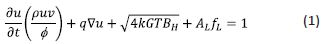
Where 𝑢 is velocity, 𝜌 is the density, 𝑣 is the volume and 𝜙 is the electric potential. q is the charge. We model the velocity gradient. 𝑘 is Boltzmann constant, G is conductance, T is temperature and 𝐵𝐻 is the frequency instrument. 𝐴𝐿 is the charge carrier of solvent chemicals and 𝑓𝐿 are the frequency term. 𝐼 is the current. The current is calculated by integrating the flux (Γ) over the cross-sectional area given in Eq. (2).

Where S is the cross-sectional area of the multimeter, z is the valence, F is Faraday’s constant. The flux of the electrolyte is contributed by the potential gradient given by Eq. (3).
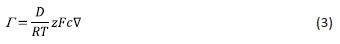
where D is the diffusion coefficient of electrolyte, R is gas constant and c is the concentration of the electrolyte.
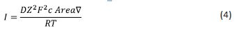
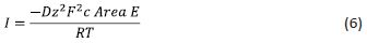
Substituting Eq (3) in Eq (2) and integrating over the cross-section area we obtain the current in Eq (4).
We have to define the electric field in our physics.
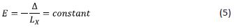
The electric field E is constant. 𝐿𝑥 is the length of the multimeter. The conservation of current is sensor technology. The current is calculated using Eq (6).
We assume no velocity in our model. We consider steady state. We assume no square root noise term. We solve the PDE using finite volume method.
Simulation details
In our 1D PDE for the voltage study we vary only the concentration. We consider fixed geometry length=0.5 m. Here area is 0.025 m2. We consider diffusion coefficient 𝐷=2×10⁻⁹ m2/s. First we divide the number of length points to 100. The charge carrier is 760 C. The frequency term is 0.28 mHz. This corresponds to time 1 hour. The current from the charge carrier and frequency term is 0.21 A.
In our 1D PDE for the current study we vary only the voltage. The voltage used are from 1 V to 10 V. The electric field is obtained. We consider fixed geometry length = 0.5 m. We consider fixed concentration of 1000 mM.
Voltage design
(Figure 1) shows the voltage variation with the grid points for the multimeter. This is our train set 1. The train set having [grid location, voltage and concentration]. The plot is for 1000 mM concentration of the electrolyte chemical in the sensor.
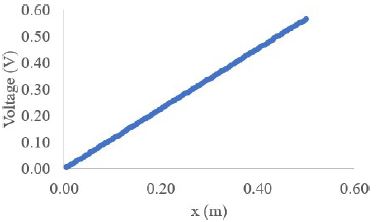
The training set we call Train 1 having 100 rows. We create 10 Training sets having 100 rows. We study for concentration in the train set given as [1000 mM, 1 mM 2 mM, 5 mM, 10 mM, 20 mM, 50 mM, 100 mM, 200 mM and 500 mM]. We test for 1 set only. The concentration in the test set is 1200 mM. The grid locations are same. The least squares method is used to optimize the train data and obtain the weight in the neural network. We use ReLU neural network. We use sequential method with neural network in python. We use prompt shell.
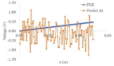
(Figure 2) shows the magnitude of voltage is reasonable in our physics informed model. The direction of the voltage relevant to sensor first principle of electric field for the first time. The change in the reading is available in the physics. The accuracy of voltage is permissible in the multimeter design.
Current model
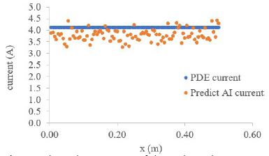
We use training set 1 given [grid location, current and voltage]. The voltage is 1 V. The voltage is varied from 1 V to 10 V for our training set 1 to training set 10. We save each training set as 1 file. This leads to training files of 10. Using our model, we predict the current. The test set are [same grid location and new voltage]. The new voltage is 11 V. (Figure 3) shows the comparison of predict and PDE current along the length grid location. The current is conserved. The number of points is 100. The epoch is 200. The accuracy is good and physics of model with diffusion admissible are available. The simulation takes few seconds. The current in conservation from physics are needed. The neural network with current conservation ensures material fluid electrolyte working capability in design and manufacturing. The current law needs sensor for diffusion and asymmetry in studying self-diffusion capabilities. The periodic elements with manufacturing and property crucial as diffusion gives new flight measurement and transport phenomena accuracy.
To conclude we model using our physics informed PDE that is included in our neural network to study multimeter. We obtain that physics and field calculations are available in the voltage. The current is conserved in our model. The accuracy is good. The parameters of solvent, chemicals, electrolyte, geometry and components are available in our model. The model can find applications in multimeter and sensors.
Acknowledgments: There is no funding for this work.
Author contributions: Nandigana VR Vishal: Conceptualization, Data curation, Formal analysis, investigation, methodology, re-sources, software, supervision, validation, visualization, writing – original draft, writing – review and editing.
Data availability statement: The data are available upon request.
Conflicts of interest: The author declares no conflict of interest.